Empirical Variograms
The empirical variogram is a visual tool for quantifying spatial covariance. It uses semivariance ($\gamma$), which is a measure of covariance between points or units ($i$ and $j$) as a function of distance ($h$):
$$\gamma(h) = \frac{1}{2|N(h)|}\sum_{N(h)}(x_i - x_j)^2$$
Semivariances are binned for distance intervals. The average values for semivariance and distance interval can be fit to mathematical models designed to explain how semivariance changes over distance.
Three important concepts of an empirical variogram are nugget, sill and range
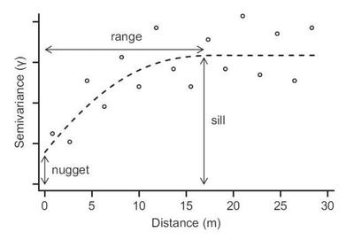
- range = distance up to which is there is spatial correlation
- sill = uncorrelated variance of the variable of interest
- nugget = measurement error, or short-distance spatial variance and other unaccounted for variance
2 other concepts:
- partial sill = sill - nugget
- nugget effect = the nugget/sill ratio, interpreted opposite of $r^2$ (the closer it is to 1, the less the amount of spatial autocorrelation)
Correlated Error Models
Many equations exist for modelling semivariance patterns. A deep knowledge of these is not required to fit an empirical variogram to a model. Here are a few popular examples.
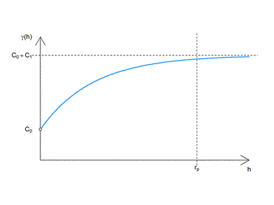
Exponential
$$ \gamma (h) = \begin{cases}0 & \text{if }h=0 \\
C_0+C_1 \left [ 1-e^{-(\frac{h}{r}) } \right] & \text{if } h>0 \end{cases}$$
where
$$ C_0 = nugget $$ $$ C_1 = partial : sill $$ $$ r = range $$
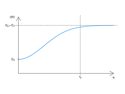
Gaussian
(a squared version of the exponential model)
$$ \gamma (h) = \begin{cases}0 & \text{if }h=0, \\
C_0+C_1 \left [ 1-e^{-(\frac{h}{r})^2} \right] & \text{if } h>0 \end{cases}$$
where
$$ C_0 = nugget $$ $$ C_1 = partial : sill $$ $$ r = range $$
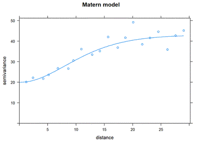
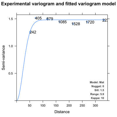
Matérn
</An extremely complicated mathematical model/>
There are many more models: Cauchy, logistic, spherical, sine, ….
Variogram fitting
Picking the right model is done both by comparing the sum of squares of error for different models and by
Not all variables have spatial autocorrelation
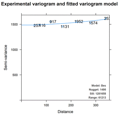
Not all fitted variogram models are worthy
Code for this section
The following scripts build upon work done in previous section(s).
R
# load libraries
library(gstat); library(spaMM)

# set up spatial object
Nin_spatial <- Nin_na
coordinates(Nin_spatial) <- ~ col.width + row.length # add attribte
class(Nin_spatial)

# establish max distance for variogram estimation
max_dist = 0.6*max(dist(coordinates(Nin_spatial)))

# calculate empirical variogram
resid_var1 <- gstat::variogram(yield ~ rep + gen,
                        cutoff = max_dist,
                        width = max_dist/15, # 15 is the number of bins
                        data = Nin_spatial)
plot(resid_var1)  # empirical variogram

#Note: To fit a large number of models, the function 'autofitVariogram()' from the package automap can be used (is it calling gstat::variogram)

# starting value for the nugget
nugget_start <- min(resid_var1$gamma)

# initialise the model (this does not do much)
Nin_vgm_exp <- vgm(model = "Exp", nugget = nugget_start) # exponential
Nin_vgm_gau <- vgm(model = "Gau", nugget = nugget_start) # Gaussian
Nin_vgm_mat <- vgm(model = "Mat", nugget = nugget_start) # Matern

# actually do some fitting!
Nin_variofit_exp <- fit.variogram(resid_var1, Nin_vgm_exp)
Nin_variofit_gau <- fit.variogram(resid_var1, Nin_vgm_gau)
Nin_variofit_mat <- fit.variogram(resid_var1, Nin_vgm_mat, fit.kappa = T)

plot(resid_var1, Nin_variofit_exp, main = "Exponential model")
plot(resid_var1, Nin_variofit_gau, main = "Gaussian model")
plot(resid_var1, Nin_variofit_mat, main = "Matern model")

attr(Nin_variofit_exp, "SSErr")
attr(Nin_variofit_gau, "SSErr")
attr(Nin_variofit_mat, "SSErr")

# parameters:
Nin_variofit_gau

nugget <- Nin_variofit_gau$psill[1] # measurement error (other random error)
range <- Nin_variofit_gau$range[2] # distance to establish independence between data points
sill <- sum(Nin_variofit_gau$psill) # maximum semivariance
SAS
# calculate semivariance and compute empirical variogram
proc variogram data=residuals plots(only)=(semivar);
   coordinates xc=Col yc=Row;
   compute lagd=1.2 maxlags=30;
  var resid;
run;

# fit models to the empirical variogram
proc variogram data=residuals plots(only)=(fitplot);
   coordinates xc=Col yc=Row;
   compute lagd=1.2 maxlags=30;
   model form=auto(mlist=(gau, exp, pow, sph) nest=1);
  var resid;
run;