Modelling Spatial Trends
The spatial models introduced in this workshop assume that spatial variation is localised and within a trial, plots located sufficiently far apart are independent of each other with no apparent spatial correlation. However, sometimes that is accurately describe a field trial. There can be experiment-wide gradients due to position on a slope, proximity to an influential environmental factor (e.g. a road), and so on. In these instances, those gradients should be modelled as a trend.
Blocking
Blocking is one example of modelling an experiment wide-trend:
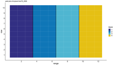
The expectation is that each block will capture and model existing variation within it. This becomes difficult to justify as blocks become large.
Rows & Ranges
Recall the RCBD model from the previous section:
$$Y_ij = \mu + \alpha_i + \beta_j + \epsilon_{ij}$$
Trials rows and ranges can likewise be modelled directly through expansion of that model (and omitting block since it full represented by column):
$$Y_ijk = \mu + \alpha_i + \beta_j + \gamma_k + \epsilon_{ijk}$$
$Y_ij$ is the independent variable
$\mu$ is the overall mean
$\alpha_i$ is the effect due to the $i^{th}$ treatment
$\beta_j$ is the effect due to the $j^{th}$ row
$\gamma_k$ is the effect due to the $k^{th}$ range (or column)
$\epsilon_{ij}$ are the error terms distributed as $N ~\sim (0,\sigma)
Code for Trends
The following scripts build upon work done in previous section(s).
R
# load libraries
library(lme4)

# exploratory plots
boxplot(yield ~ rep, data = Nin, xlab = "block", col = "red2")
boxplot(yield ~ row, data = Nin, xlab = "row", col = "dodgerblue2")
boxplot(yield ~ col, data = Nin, xlab = "column", col = "gold")

## row/column model ##

# data prep
Nin$rowF = as.factor(Nin$row)
Nin$colF = as.factor(Nin$col)

# specify model
nin.rc <- lmer(yield ~ gen + (1|colfF) + (1|rowF),
              data = Nin, na.action = na.exclude)
# extract random effects for row and column
ranef(nin_rc)
# extract predictions
nin_rc <- as.data.frame(emmeans(nin.rc, "gen"))
SAS
# exploratory boxplots
proc sgplot data=alliance;
    vbox yield/category=rep FILLATTRS=(color=red) LINEATTRS=(color=black) WHISKERATTRS=(color=black);
run;

proc sgplot data=alliance;
    vbox yield/category=Col FILLATTRS=(color=yellow) LINEATTRS=(color=black) WHISKERATTRS=(color=black);
run;

proc sgplot data=alliance;
    vbox yield/category=Row FILLATTRS=(color=blue) LINEATTRS=(color=black) WHISKERATTRS=(color=black);
run;

# row/column model
proc mixed data=alliance ;
	class entry rep;
	model yield = entry  row col/ddfm=kr;
	random rep;
	lsmeans entry/cl;
	ods output LSMeans=NIN_row_col_means;
	title1 'NIN data: RCBD';
run;
Splines
Polynomial splines are an additional method for spatial adjustment and represent a more non-parametric method that does not rely on estimation or modeling of variograms. Instead, it uses the raw data and residuals to fit a surface to the spatial data and adjust the variance covariance matrix accordingly.
Code for Splines
The following scripts build upon work done in previous section(s).
R
nin_spline <- SpATS(response = "yield",
                    spatial = ~ PSANOVA(col, row, nseg = c(10,20),
                                        degree = 3, pord = 2),
                    genotype = "gen",
                    random = ~ rep, # + rowF + colF,
                    data = Nin,
                    control = list(tolerance = 1e-03, monitoring = 0))

preds_spline <- predict(nin_spline, which = "gen") %>%
  dplyr::select(gen, emmean = "predicted.values", SE = "standard.errors")
SAS
proc glimmix data=alliance ;
    class entry rep;
    effect sp_r = spline(row col);
    model yield = entry  sp_r/ddfm=kr;
    random row col/type=rsmooth;
    lsmeans entry/cl;
    ods output LSMeans=NIN_smooth_means;
    title1 'NIN data: RCBD';
run;