Diagnosing Spatial Autocorrelation

Spatial autocorrelation refers to similarity between points that are close to one another. That correlation is expected to decline with distance. Note that is different from experiment-wide gradients, such as a salinity gradient or position on a slope.

Plotting

One of the easiest ways to diagnose spatial autocorrelation is by plotting data by its spatial position and using a heat map to indicate values of a response variable.

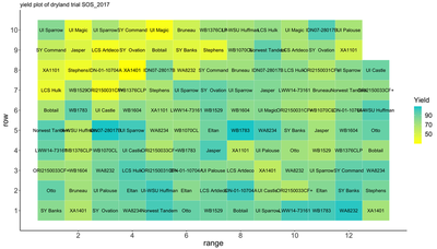
While there is always ambiguity associated with using plots for decision making, early exploration of these plots can be helpful in understanding the extent of spatial correlation.

Moran’s I

Moran’s I, sometimes called “Global Moran’s I” can be used for conducting a hypothesis test on whether there is correlation between spatial units located adjacent to one another.

$$ I = \frac{N}{W}\frac{\sum_i \sum_j w_{ij} (x_i - \bar{x})(x_j - \bar{x})}{\sum_i(x_i - \bar{x})^2} \qquad i \neq j$$

Where N is total number of spatial locations indexed by $i$ and $j$, x is the variable of interest, $w_{ij}$ are a spatial weights between each $i$ and $j$, and W is the sum of all weights.

The expected values of Moran’s I is $-1/(N-1)$. Values greater than the expected value indicate positive spatial correlation (areas close to each other are similar), while values less than that indicate dissimilarity as spatial distance between points decreases.

Defining Neighbors

There are several options for defining adjacent neighbors and how to weight each neighbor’s influence. The two common configurations for defining neighbors are the rook and queen configurations. These are exactly what their chess analogy suggests: “rook” defines neighbors in an row/column fashion, while “queen” defines neighbors in a row/column configuration an also neighbors located diagonally at a 45 degree angle from the row/column neighbors. Determining this can be complicated when working with irregularly-placed data (e.g. counties), but is quite unambiguous for lattice data common in planned field experiments.

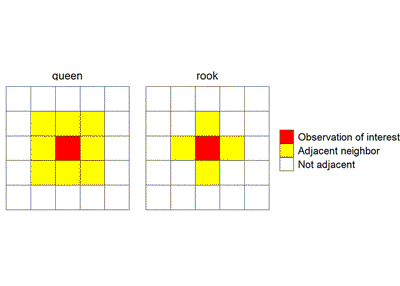
Setting the values for weights is a function of both how neighbors are defined and their proximity to the unit of interest. However, a very popular method is to define each neighbor as equal fractions that sum to one, e.g. in rook formation, each neighbor is weighted 0.25 (assuming an interior plot with 4 neighbors).

Empirical variogram

This is one of the most useful methods of determining the extent of spatial variability and will be covered in the following sections.

Code for this section

# load libraries
library(dplyr); library(ggplot2); library(desplot); 
library(spdep); library(sf); library(nlme)

# read in data and prepare it
Nin <- read.csv("stroup_nin_wheat.csv") %>% 
  mutate(col.width = col * 1.2, row.length = row * 4.3) %>% 
  mutate(name = case_when(is.na(as.character(rep)) ~ NA_character_, 
                          TRUE ~ as.character(gen))) %>% 
  arrange(col, row)

Nin_na <- filter(Nin, !is.na(rep))

# make exploratory plot
ggplot(Nin, aes(x = row, y = col)) +
  geom_tile(aes(fill = yield), col = "white") +
  geom_tileborder(aes(group = 1, grp = rep), lwd = 1.2) +
  labs(x = "row", y = "column", title = "field plot layout") + 
  theme_classic() +
  theme(axis.text = element_text(size = 12),
        axis.title = element_text(size = 14),
        legend.title = element_text(size = 14),
        legend.text = element_text(size = 12))

## conduct moran's I test ##

# set neighbors with convenience function for grids
xy_rook <- cell2nb(nrow = max(Nin$row), ncol = max(Nin$col), 
  type="rook", torus = FALSE, legacy = FALSE)  

# run linear mixed model and extract residuals
nin.lme <- lme(fixed = yield ~ gen, random = ~1|rep,
              data = Nin, na.action = na.exclude)
resid_lme <- residuals(nin.lme)
names(resid_lme) <- Nin$plot

# two version of the Moran's I test: 
moran.test(resid_lme, nb2listw(xy_rook), na.action = na.exclude)
moran.mc(resid_lme, nb2listw(xy_rook), 999, na.action = na.exclude)

# read in data
proc format;
  invalue has_NA
  'NA' = .;
;

filename NIN url "https://raw.githubusercontent.com/IdahoAgStats/guide-to-field-trial-spatial-analysis/master/data/stroup_nin_wheat.csv";

data alliance;
    infile NIN firstobs=2 delimiter=',';
    informat yield has_NA.;
    input entry $   rep $   yield   col row;
    Row  = 4.3*Row;
    Col = 1.2*Col;
    if yield=. then delete;
run;

# heatmap
proc sgplot data=alliance;
    HEATMAPPARM y=Row x=Col COLORRESPONSE=yield/ colormodel=(blue yellow green); 
run;

# linear mixed model
proc mixed data=alliance;
   class Rep Entry;
   model Yield = Entry / outp=residuals;
   random Rep;
run;

# Moran's I
proc variogram data=residuals plots(only)=moran ;
   compute lagd=1.2 maxlag=30 novariogram autocorr(assum=nor) ;
   coordinates xc=row yc=col;
   var resid;
run;