How to Write Custom Functions in R

You may find yourself needing to do something repeatedly in R. Sure, you can cut-and-paste and change that one thing, or two things, or five things, but this quickly becomes cumbersome. The result can be a very long R file and the likelihood of making a mistake that you don’t notice increases (e.g. forgetting to change a variable or an argument).

There is the general rule of DRY: don’t repeat yourself. In practice, if something has to pasted more than twice, then consider writing a function to accomplish that aim instead.

Introduction to Writing Functions

R functions follow a general structure:

my_function_name <- function(argument1, argument2) {
  final_output <- action(argument1, argument2)
  return(final_output)
}

A classic function example is conversion of temperature from Fahrenheit to celsius:

fahr_to_cel <- function(fahr) {
  # function that converts temperature in degrees Fahrenheit to celsius
  # input: fahr: numeric value representing temp in degrees fahrenheit
  # output: kelvin: numeric converted temp in celsius
  celsius <- ((fahr - 32) * (5 / 9)) 
  return(celsius)
}

This function takes a numeric value, temperature in Fahrenheit, and outputs another numeric value, that same value converted to celsius.

Function usage:

fahr_to_cel(80)

## [1] 26.66667

This function can be called for a large number of values at once:

# create a vector of 100 numbers randomly sampled between 1 and 100. 
x1 <- sample(1:100, 100, replace = TRUE)
x2 <- fahr_to_cel(x1)

If you provide the incorrect type of data, the function will not work:

fahr_to_cel("thirty")

## Error in fahr - 32: non-numeric argument to binary operator

A More Complex Example

Often we want to do something more complicated. One thing I want to do frequently is build boxplots.

First, simulate some data. This data set has two categorical variables, cat1 and cat2, and 4 different continuous variables generated through data simulation.

mydata <- data.frame(cat1 = rep(c("A", "B", "C", "D"), 10),
                     cat2 = rep(c("one", "two"), each = 20),
                     var1 = rnorm(40),
                     var2 = runif(40), 
                     var3 = rlnorm(40),
                     var4 = rbeta(40, 1, 5))

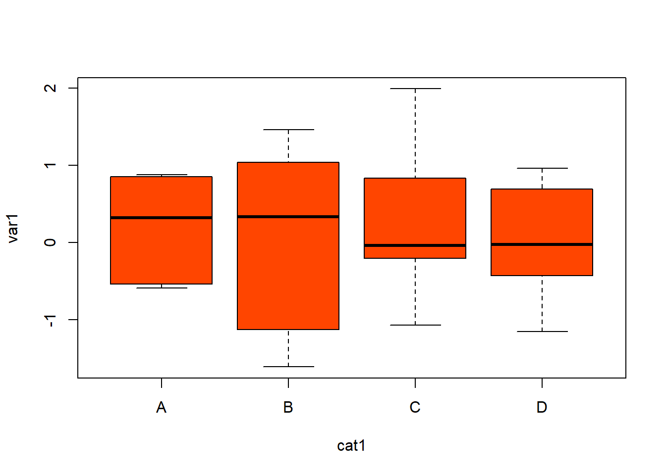
Next, write up an example of what you want to do. In this example, let’s create a boxplot:

boxplot(var1 ~ cat1, data = mydata,
        main = NA, col = "orangered")

Now, let’s put that in a function. Start with the basic function framework:

boxplot_func = function() {

}

Next, insert the function code. Start by cut-and-pasting the original boxplot command ran above:

boxplot_func = function() {
    boxplot(var1 ~ cat1, data = mydata,
    main = NA, col = "orangered")
}

Decide on arguments you want to control and put that inside the function() parentheses. Probably the independent and dependent variable (x and y, respectively), as well as the data frame needed.

Put those arguments inside function().

boxplot_func = function(df, x, y) {
    boxplot(var1 ~ cat1, data = mydata,
    main = NA, col = "orangered")
}

Then indicate where those arguments are used in the function. They must be used in the function (otherwise, why have them?).

boxplot_func = function(df, x, y) {
    boxplot(y ~ x, data = df,
    main = NA, col = "orangered")
}

However, if you try to use this function, it won’t work. The argument y ~ x is a special class of object in R called “formula” and the formatting and object type must match. Formulas are used widely in R for linear modelling and follow the exact same convention:

y ~ x  

Note that the information on either side of ~ can become more complicated. (but not in this function).

So, create a formula object using the functions formula() and paste() within the function and insert that into the basic boxplot code. If you don’t know how to use those function, type ?formula and ?paste into the console to learn more about them.

boxplot_func = function(df, x, y) {
    f = formula(paste(y, "~", x))
    boxplot(f, data = df,
    main = NA, col = "orangered")
}

What if you want the ability to change the color? Insert a new argument and replace it in the function body:

boxplot_func = function(x, y, color) {
    f = formula(paste(y, "~", x))
    boxplot(f, data = df,
    main = NA, col = color)
}

If you want the option to set the some options or if you choose not to, have the function choose values automatically as defaults, that can be done by naming the argument in formula().

boxplot_func = function(df = mydata, x, y, color = "springgreen") {
    f = formula(paste(y, "~", x))
    boxplot(f, data = df,
    main = NA, col = color)
}

Next step is to run the function as it is currently written (highlight the function code and click run). Next, make sure you add this function (i.e. boxplot_funct = function(...)) to your R environment by running it in the console. You can check it exists in your R global environment as thus:

ls()

## [1] "boxplot_func" "fahr_to_cel"  "mydata"       "x1"           "x2"

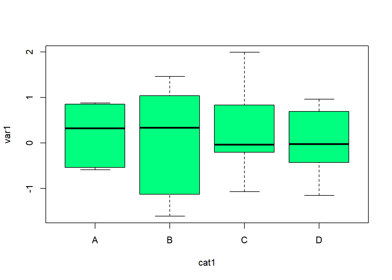
Now, call the function and make sure it does what we want?

boxplot_func(mydata, "cat1", "var1")

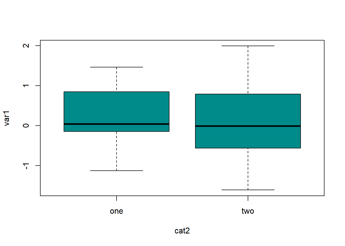
boxplot_func(x = "cat2", y = "var1", col = "darkcyan")

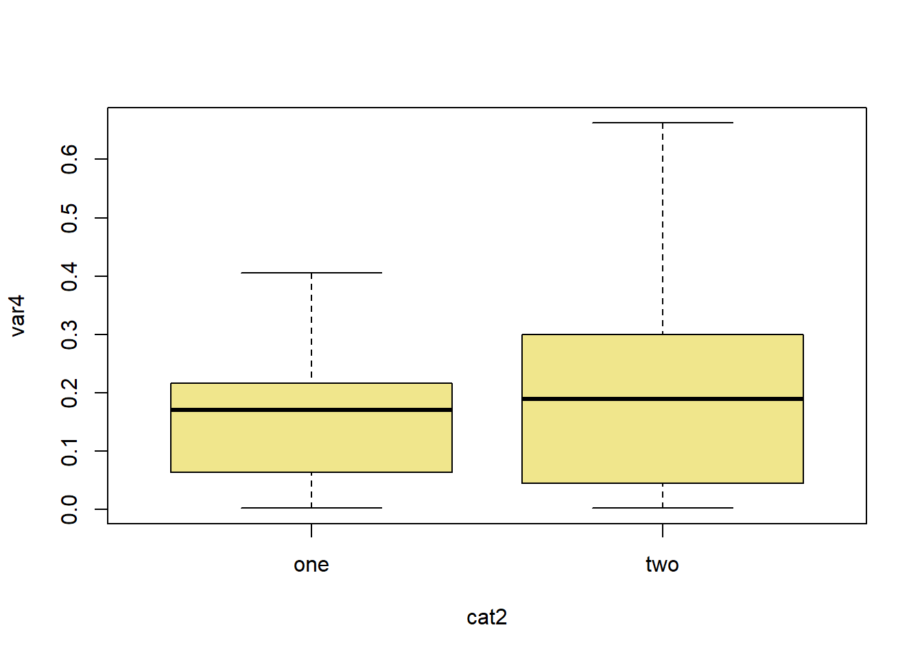
boxplot_func(mydata, "cat2", "var4", col = "khaki")

What if it doesn’t do what we want? What if you get strange output? No output? Or strange error messages? Herein comes the world of debugging (another blog post for another day).

Error Checking and Error Messages

You may have noticed earlier this strange error message:

fahr_to_cel("thirty")

## Error in fahr - 32: non-numeric argument to binary operator

This is a very confusing message. We most certainly provided a “non-numeric argument”, but what is a “binary operator”? Turns out that is a programming speak for a standard mathematical operations addition, subtraction, multiplication and division (called ‘binary’ because they take two inputs). Still, we are likely to encounter more strange error messages written in programmer speak that confuse us or someone else using our functions. We can write custom error messages that are produced when certain errors occur.

Here is the temperature conversion function again:

fahr_to_cel <- function(fahr) {
  celsius <- ((fahr - 32) * (5 / 9)) 
  return(celsius)
}

Since they can only take numeric argument, maybe we can start for checking for this? There are a few options in do this. One of the easiest to use is stopifnot(). This functions takes the general form: stopifnot("my custom error message" = test). What constitutes a ‘test’ is an R expression that returns a TRUE or FALSE value after being evaluated. Examples of this are is.character(x), is.NA(x), x > 0 and so on. For each of these statements, the expectation is that R will true a TRUE or FALSE. If the test does not do this reliably (e.g. you may not be able to evaluate x > 0 if x is non-numeric), then a different test is needed.

In our case, we can use is.numeric().

fahr_to_cel <- function(fahr) {
  stopifnot("input is not numeric" = is.numeric(fahr))
  celsius <- ((fahr - 32) * (5 / 9)) 
  return(celsius)
}

Let’s run some test cases:

fahr_to_cel(30)

## [1] -1.111111

fahr_to_cel("thirty")

## Error in fahr_to_cel("thirty"): input is not numeric

As expected, the first one worked and the second generated an error message.

Naturally, this is a very trivial example, but if you write more complicated functions with the intent of them automatically accomplishing a goal for you, these error messages can be helpful.

Functions and Tidy Evaluation

If you’ve worked with the tidyverse, you know it handles input a bit differently. In summary, quotes are used far less often. This makes writing function quite challening at times and required the use of the double curly braces, {{}} or the “bang-bang” operator !!.

What if we wanted to do a boxplot function using ggplot?

Here’s what the code would look like:

library(ggplot2)

mydata <- data.frame(cat = rep(c("AA", "BB"), each = 50), 
                     obs = c(rnorm(50), runif(50)))

ggplot(mydata, aes(x = cat, y = obs)) +
  geom_boxplot(aes(fill = cat), alpha = 0.5) +
  geom_jitter(height = 0, width = 0.2, alpha = 0.6, color = "black") + 
  guides(fill = "none") +
  theme_classic()

But, if you try to write a function following the usual rules, it won’t work properly:

gboxplot_func <- function(x1, y1) {
  ggplot(mydata, aes(x = x1, y = y1)) +
  geom_boxplot(aes(fill = x1), alpha = 0.5) +
  geom_jitter(height = 0, width = 0.2, alpha = 0.6, color = "black") + 
  guides(fill = "none") +
  theme_classic()
}

gboxplot_func(cat, obs)

## Error in FUN(X[[i]], ...): object 'obs' not found

This one works, but the results are crazy.

gboxplot_func("cat", "obs")

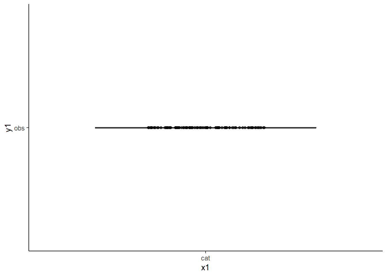
Why are the results wonky? Because while this function see “mydata” has 100 observations, it cannot connect “cat” and “obs” to the data frame.

This is where the special operators come in:

gboxplot_func2 <- function(x1, y1) {
  ggplot(mydata, aes(x = {{x1}}, y = {{y1}})) +
  geom_boxplot(aes(fill = {{x1}}), alpha = 0.5) +
  geom_jitter(height = 0, width = 0.2, alpha = 0.6, color = "black") + 
  guides(fill = "none") +
  theme_classic()
}

gboxplot_func2(cat, obs)

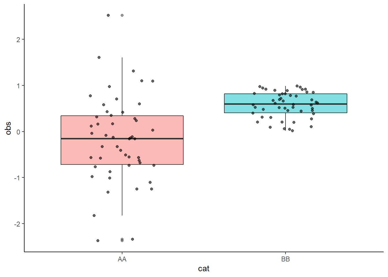
The curly braces enable us to insert unquoted tidy variables and use ggplot.

What if you have multiple options to specify in a single arguments? You can use the ... notation (in the final argument):

var_sum_funct(storms, day, name)[1:5,] # one grouping factor

## # A tibble: 5 × 3
##   name      Mean     SD
##   <chr>    <dbl>  <dbl>
## 1 AL011993  8.75 13.7  
## 2 AL012000  7.75  0.5  
## 3 AL021992 25.6   0.548
## 4 AL021994 20.3   0.516
## 5 AL021999  2.75  0.5

var_sum_funct(storms, day, name, status)[1:5,] # many grouping factors

## `summarise()` has grouped output by 'name'. You can override using the
## `.groups` argument.

## # A tibble: 5 × 4
## # Groups:   name [5]
##   name     status               Mean     SD
##   <chr>    <chr>               <dbl>  <dbl>
## 1 AL011993 tropical depression  8.75 13.7  
## 2 AL012000 tropical depression  7.75  0.5  
## 3 AL021992 tropical depression 25.6   0.548
## 4 AL021994 tropical depression 20.3   0.516
## 5 AL021999 tropical depression  2.75  0.5

var_sum_funct(storms, day) # unusual example! 

## # A tibble: 1 × 2
##    Mean    SD
##   <dbl> <dbl>
## 1  15.8  8.94

This is a very brief introduction to tidy evaluation. More information on tidy evaluation is available for ggplot and dplyr.