Applied ANOVA in R
Navigating the R linear model wilderness

Introduction
ANOVA in R is a unfortunately a bit complicated. Unlike SAS, ANOVA functions in R lack a consistent structure, consistent output and the accessory packages for ANOVA display a patchwork of compatibility. The result is that it is easy to misspecify a model or make other mistakes. The information below is intended to serve as a guide through the R ANOVA wilderness.
Packages Needed
There are many packages to load. Here is a (very) brief summary of what each package does.
| Package | Purpose |
|---|---|
| car | Anova() function to extract type III & II sums of squares |
| lme4 | mixed models |
| nlme | mixed models, non-linear models, alternative covariance structures |
| emmeans | for extracting least squares means and contrasts |
| lmer test | improved summary functions of lmer objects |
| dplyr | data organization |
| forcats | for managing categorical data |
| agridat | has many agricultural data sets |
| agricolae | has options for many common agricultural experimental designs |
library(car)
library(lme4)
library(nlme)
library(emmeans) #in older version of R, you may need to install "multcompView" separately to access full functionality of the emmeans package
library(lmerTest)
library(dplyr)
library(forcats)
library(agridat)
Formula Notation
There are some consistent features across ANOVA methods in R. Formula notation is often used in the R syntax for ANOVA functions. It looks like this: $Y ~ X, where Y is the dependent variable (the response) and X is/are the independent variable(s) (e.g. the experimental treatments).
my_formula <- formula(Y ~ treatment1 + treatment2)
class(my_formula)
## [1] "formula"
my_formula
## Y ~ treatment1 + treatment2
Often the independent variables (i,e, the treatments or the x variables) are expected to be factors, another type of R object:
my_var <- c(rep("low",5), rep("high", 5))
class(my_var) #check what variable type it is
## [1] "character"
Although “my_var” is not type factor, it is type “character” which is automatically converted to a factor in lm(), lmer(), lme() and many other linear modeling functions. There are some packages that do not follow this convention, so it’s helpful to read function documentation, especially if you get unexpected results.
Variables like year, which are often imported as a number or integer, do need to be converted to a factor or a character variable prior to analysis. Otherwise, they will be interpreted as a number in linear modelling and treated as a covariate, e.g, 2020 would be 2,020. Here is one way to do this conversion:
my_factor <- as.character(my_var) # convert to a character
class(my_factor) # check variable type to confirm
## [1] "character"
my_factor <- as.factor(my_var) # convert to a factor
class(my_factor) # check variable type again to confirm
## [1] "factor"
The choice of whether to convert a categorical variable to a character or factor depends on the comfort of the user with these structures and package requirements.
Sometimes, there is a need to alter the order of treatment levels (that is, how R sees those levels). The default behavior of R is to order categorical levels alphanumerically. However, sometimes there are reasons you may not want this (for example, you want to set a particular reference level as the first factor level).
Below is one example of how to reorder factor levels in a variable. The first step is to see which levels are present in the variable and how they are ordered:
levels(my_factor)
## [1] "high" "low"
Once that is known, you can use that information to manually set the levels and their order. Note that spelling of each level much match what is actually present in the variable. Unmatched levels in the variable will be set to NA automatically by R in the following step.
my_factor <- factor(my_factor, levels = c("low", "high"))
levels(my_factor) # check the new ordering
## [1] "low" "high"
Knowing the level order is important because in the implementation of ANOVA in R, the first level is treated as the reference level. Manipulating factors is a challenging task in R. The package forcats contains a collection of accessory functions for managing factors (“forcats” = for categories). The tutorial uses the forcats function fct_drop().
More on formulas:
The formula first shown, Y ~ treatment1 + treatment2, includes main effects only. Other formula notation includes the symbols : and *, indicating notation for interaction only and main effects plus the interaction term, respectively.
formula(Y ~ treatment1:treatment2) # interaction only
## Y ~ treatment1:treatment2
formula(Y ~ treatment1*treatment2) # interaction plus main effects
## Y ~ treatment1 * treatment2
These two formulas are equivalent:
formula(Y ~ treatment1 + treatment2 + treatment1:treatment2)
formula(Y ~ treatment1*treatment2)
Perhaps you can see from these examples that formulas are a really just a collections of characters (that is, a string) and exist independent of any data set. Later, we will need to link these formulas to a data set to actually construct a linear model and conduct statistical analysis.
ANOVA for fixed effects models
Here is a function for reporting the number of missing data in each column. There are other ways to do this, but I find this function easy enough to write and use.
count_na <- function(df) {
  apply(df, 2, function(x) sum(is.na(x)))
}
Completely Randomised design
First, load the data set “warpbreaks” (a data set from base R). This is an old data set with variables for wool type (A and B) and tension on the loom (L, M or H). The response variable is “breaks”, the number of times the wool thread breaks on industrial looms.
I always like to have a quick look at the data before running any statistical tests. So, here we go:
data(warpbreaks)
count_na(warpbreaks)
##  breaks    wool tension
##       0       0       0
str(warpbreaks)
## 'data.frame':	54 obs. of  3 variables:
##  $ breaks : num  26 30 54 25 70 52 51 26 67 18 ...
##  $ wool   : Factor w/ 2 levels "A","B": 1 1 1 1 1 1 1 1 1 1 ...
##  $ tension: Factor w/ 3 levels "L","M","H": 1 1 1 1 1 1 1 1 1 2 ...
warpbreaks$wool <- factor(warpbreaks$wool, levels = c("A", "B", "C"))

table(warpbreaks$wool, warpbreaks$tension)
##
##     L M H
##   A 9 9 9
##   B 9 9 9
##   C 0 0 0
hist(warpbreaks$breaks, col = "gold")

boxplot(breaks ~ wool, data = warpbreaks, col = "orangered")

boxplot(breaks ~ tension, data = warpbreaks, col = "chartreuse") #why not have colorful plots?

This data set has 2 treatments. We don’t know if there is an interaction between the variables, yet. A good start is to run a linear model using lm() function, the linear regression function. As a reminder, ANOVA is a special case of the linear regression model where the predictors (the experimental treatments) are categories rather than a continuous variable.
# run standard linear model for main effects only
lm.mod1 <- lm(breaks ~ wool + tension, data = warpbreaks)

# extract type III sums of squares from that model
Anova(lm.mod1, type = "3")
## Anova Table (Type III tests)
##
## Response: breaks
##              Sum Sq Df  F value    Pr(>F)
## (Intercept) 20827.0  1 154.3226 < 2.2e-16 ***
## wool          450.7  1   3.3393  0.073614 .
## tension      2034.3  2   7.5367  0.001378 **
## Residuals    6747.9 50
## ---
## Signif. codes:  0 '***' 0.001 '**' 0.01 '*' 0.05 '.' 0.1 ' ' 1
# run a linear model with main effects and interactions
lm.mod2 <- lm(breaks ~ wool*tension, data = warpbreaks)

# ...and type III sums of squares
Anova(lm.mod2, type = "III")
## Anova Table (Type III tests)
##
## Response: breaks
##               Sum Sq Df  F value    Pr(>F)
## (Intercept)  17866.8  1 149.2757 2.426e-16 ***
## wool          1200.5  1  10.0301 0.0026768 **
## tension       2468.5  2  10.3121 0.0001881 ***
## wool:tension  1002.8  2   4.1891 0.0210442 *
## Residuals     5745.1 48
## ---
## Signif. codes:  0 '***' 0.001 '**' 0.01 '*' 0.05 '.' 0.1 ' ' 1
FYI
functions only shown as an example and not actually run.
# this function runs type II sums of squares:
Anova(lm.mod2, type = "II")
# this function runs type I sums of squares:
anova(lm.mod2)
A few comments on types of sums of squares:
As a reminder, the type of sums of squares used in statistical tests can impact the results and subsequent interpretation. Type I, sums of squares tests for statistical significance by adding one variable to the model at time (and hence is also called “sequential”). If there is any unbalance in the treatments, the type I sums of squares are dependent on the order variables are added to the model and hence is often not the best choice for many agricultural experiment. Type III sums of squares (also called “partial” or “marginal”) evaluates the statistical significance of variable or interaction, assuming that the other variables are in the model. This is a decent default option. The last option is Type II sums of squares, which is the best option when you are sure there are no interactions between variables. If there is complete balance among treatments (each treatment is observed the same number of times with no missing data), then there is no need to concern yourself with these different types of sums of squares.
Compare Models
# conduct an F test comparing the models
anova(lm.mod1, lm.mod2)
## Analysis of Variance Table
##
## Model 1: breaks ~ wool + tension
## Model 2: breaks ~ wool * tension
##   Res.Df    RSS Df Sum of Sq      F  Pr(>F)
## 1     50 6747.9
## 2     48 5745.1  2    1002.8 4.1891 0.02104 *
## ---
## Signif. codes:  0 '***' 0.001 '**' 0.01 '*' 0.05 '.' 0.1 ' ' 1
# also, consider doing a stepwise approach for finding the best model:
step(lm.mod2)
## Start:  AIC=264.02
## breaks ~ wool * tension
##
##                Df Sum of Sq    RSS    AIC
## <none>                      5745.1 264.02
## - wool:tension  2    1002.8 6747.9 268.71
##
## Call:
## lm(formula = breaks ~ wool * tension, data = warpbreaks)
##
## Coefficients:
##    (Intercept)           woolB        tensionM        tensionH  woolB:tensionM
##          44.56          -16.33          -20.56          -20.00           21.11
## woolB:tensionH
##          10.56
Model diagnostics
plot(lm.mod2) #this will produce 4 plots of residuals


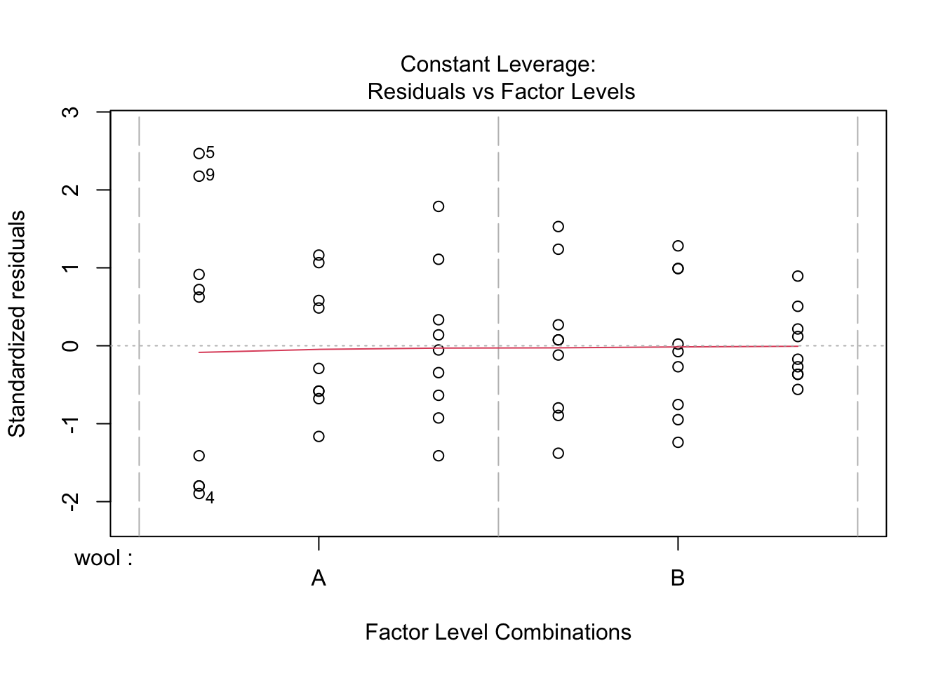
shapiro.test(resid(lm.mod2)) #standard shapiro-wilk test.
##
## 	Shapiro-Wilk normality test
##
## data:  resid(lm.mod2)
## W = 0.98686, p-value = 0.8162
# this variable could be analyzed with a log-normal model instead
Least squares means & contrasts
The emmeans package is a flexible package for extracting the estimated marginal means (in SAS, the “least squares means”) from different linear models. It is compatible with a large number of R linear modelling packages.
Here is some code for extracting the marginal means and conducting contrasts.
# extract least squares means for 'tension'
(lsm <- emmeans(lm.mod2, ~ tension))
## NOTE: Results may be misleading due to involvement in interactions
##  tension emmean   SE df lower.CL upper.CL
##  L         36.4 2.58 48     31.2     41.6
##  M         26.4 2.58 48     21.2     31.6
##  H         21.7 2.58 48     16.5     26.9
##
## Results are averaged over the levels of: wool
## Confidence level used: 0.95
emmeans(lm.mod2, "wool")
## NOTE: Results may be misleading due to involvement in interactions
##  wool emmean   SE df lower.CL upper.CL
##  A      31.0 2.11 48     26.8     35.3
##  B      25.3 2.11 48     21.0     29.5
##
## Results are averaged over the levels of: tension
## Confidence level used: 0.95
All pairwise comparisons within each level of tension:
contrast(lsm, "pairwise")
##  contrast estimate   SE df t.ratio p.value
##  L - M       10.00 3.65 48   2.742  0.0229
##  L - H       14.72 3.65 48   4.037  0.0006
##  M - H        4.72 3.65 48   1.295  0.4049
##
## Results are averaged over the levels of: wool
## P value adjustment: tukey method for comparing a family of 3 estimates
Conduct custom contrasts comparing ‘Low’ tension versus ‘Medium’ and ‘High’ and ‘High’ versus ‘Medium’ and ‘Low’.
# see the order of each level in a factor
levels(warpbreaks$tension)
## [1] "L" "M" "H"
# construct a list of constructs
# each item must be same length as the the number of levels present in the variable tension
# use numbers and fracions to indicate the contrasting levels
# the numbers must sum to zero
cList <- list(LvMH = c(1, -0.5, -0.5), # low vs high + medium
              HvLM = c(0.5, 0.5, -1))  # high vs low + medium

# check that each contrast sums to zero
lapply(cList, sum)
## $LvMH
## [1] 0
##
## $HvLM
## [1] 0
# perform custom contrast and include a Bonferroni adjustment
summary(contrast(lsm, cList, adjust = "bonferroni"))
##  contrast estimate   SE df t.ratio p.value
##  LvMH        12.36 3.16 48   3.914  0.0006
##  HvLM         9.72 3.16 48   3.078  0.0069
##
## Results are averaged over the levels of: wool
## P value adjustment: bonferroni method for 2 tests
Randomised Complete Block Design (RCBD) - fixed effects model
This example uses rapeseed yield data from multiple locations, years and cultivars. Within a single location or year, the replication is often balanced.
Load Data and examine:
data(shafii.rapeseed) # from the 'agridat' package

rapeseed1987 <- shafii.rapeseed %>% filter(year == 87) %>%
  mutate(block = fct_drop(rep), Cv = fct_drop(gen), loc = fct_drop(loc))

str(rapeseed1987)
## 'data.frame':	216 obs. of  7 variables:
##  $ year : int  87 87 87 87 87 87 87 87 87 87 ...
##  $ loc  : Factor w/ 9 levels "GGA","ID","MT",..: 1 1 1 1 1 1 1 1 1 1 ...
##  $ rep  : Factor w/ 4 levels "R1","R2","R3",..: 1 2 3 4 1 2 3 4 1 2 ...
##  $ gen  : Factor w/ 6 levels "Bienvenu","Bridger",..: 1 1 1 1 2 2 2 2 3 3 ...
##  $ yield: num  961 1329 1781 1698 1605 ...
##  $ block: Factor w/ 4 levels "R1","R2","R3",..: 1 2 3 4 1 2 3 4 1 2 ...
##  $ Cv   : Factor w/ 6 levels "Bienvenu","Bridger",..: 1 1 1 1 2 2 2 2 3 3 ...
count_na(rapeseed1987)
##  year   loc   rep   gen yield block    Cv
##     0     0     0     0     0     0     0
table(rapeseed1987$Cv, rapeseed1987$loc) #experiment has 1 rep per block
##
##            GGA ID MT NC OR SC TGA TX WA
##   Bienvenu   4  4  4  4  4  4   4  4  4
##   Bridger    4  4  4  4  4  4   4  4  4
##   Cascade    4  4  4  4  4  4   4  4  4
##   Dwarf      4  4  4  4  4  4   4  4  4
##   Glacier    4  4  4  4  4  4   4  4  4
##   Jet        4  4  4  4  4  4   4  4  4
hist(rapeseed1987$yield, col = "gold")

boxplot(yield ~ Cv, data = rapeseed1987, col = "orangered")

boxplot(yield ~ loc, data = rapeseed1987, col = "chartreuse")

Analyse experiment:
# for this example, the analysis will only be done for a single year
# block is nested within location
# if each block had a unique name, 'Error(block)' would suffce
shaf.aov <- aov(yield ~ Cv*loc + Error(block), data = rapeseed1987)

summary(shaf.aov)
##
## Error: block
##           Df Sum Sq Mean Sq F value Pr(>F)
## Residuals  3 336565  112188
##
## Error: Within
##            Df    Sum Sq  Mean Sq F value   Pr(>F)
## Cv          5   3203992   640798   2.645 0.025111 *
## loc         8 318197192 39774649 164.165  < 2e-16 ***
## Cv:loc     40  22707425   567686   2.343 0.000103 ***
## Residuals 159  38523267   242285
## ---
## Signif. codes:  0 '***' 0.001 '**' 0.01 '*' 0.05 '.' 0.1 ' ' 1
emmeans(shaf.aov, ~ Cv | loc)
## Note: re-fitting model with sum-to-zero contrasts
## loc = GGA:
##  Cv       emmean  SE  df lower.CL upper.CL
##  Bienvenu   1442 245 161      959     1926
##  Bridger    1363 245 161      880     1847
##  Cascade    1505 245 161     1021     1988
##  Dwarf      1295 245 161      811     1779
##  Glacier    1681 245 161     1197     2164
##  Jet        1091 245 161      607     1575
##
## loc = ID:
##  Cv       emmean  SE  df lower.CL upper.CL
##  Bienvenu   1242 245 161      759     1726
##  Bridger     947 245 161      463     1430
##  Cascade     773 245 161      290     1257
##  Dwarf       932 245 161      448     1415
##  Glacier    1111 245 161      627     1595
##  Jet        1064 245 161      580     1548
##
## loc = MT:
##  Cv       emmean  SE  df lower.CL upper.CL
##  Bienvenu   2616 245 161     2132     3100
##  Bridger    2828 245 161     2345     3312
##  Cascade    2916 245 161     2433     3400
##  Dwarf      3452 245 161     2968     3935
##  Glacier    3307 245 161     2823     3790
##  Jet        3660 245 161     3177     4144
##
## loc = NC:
##  Cv       emmean  SE  df lower.CL upper.CL
##  Bienvenu   1001 245 161      517     1485
##  Bridger    1064 245 161      581     1548
##  Cascade     745 245 161      262     1229
##  Dwarf      1014 245 161      530     1497
##  Glacier    1229 245 161      746     1713
##  Jet        1674 245 161     1190     2157
##
## loc = OR:
##  Cv       emmean  SE  df lower.CL upper.CL
##  Bienvenu   4556 245 161     4072     5039
##  Bridger    2530 245 161     2046     3013
##  Cascade    3336 245 161     2852     3819
##  Dwarf      3932 245 161     3448     4415
##  Glacier    4185 245 161     3702     4669
##  Jet        3220 245 161     2736     3703
##
## loc = SC:
##  Cv       emmean  SE  df lower.CL upper.CL
##  Bienvenu   2500 245 161     2016     2983
##  Bridger    2705 245 161     2221     3189
##  Cascade    2119 245 161     1635     2602
##  Dwarf      1894 245 161     1410     2377
##  Glacier    2717 245 161     2234     3201
##  Jet        2833 245 161     2349     3316
##
## loc = TGA:
##  Cv       emmean  SE  df lower.CL upper.CL
##  Bienvenu   1258 245 161      774     1741
##  Bridger    1868 245 161     1384     2351
##  Cascade    1708 245 161     1224     2191
##  Dwarf       873 245 161      389     1356
##  Glacier    1453 245 161      970     1937
##  Jet         954 245 161      470     1438
##
## loc = TX:
##  Cv       emmean  SE  df lower.CL upper.CL
##  Bienvenu    838 245 161      354     1322
##  Bridger    1069 245 161      585     1553
##  Cascade     735 245 161      251     1218
##  Dwarf       988 245 161      505     1472
##  Glacier     952 245 161      468     1435
##  Jet        1408 245 161      925     1892
##
## loc = WA:
##  Cv       emmean  SE  df lower.CL upper.CL
##  Bienvenu   4375 245 161     3891     4859
##  Bridger    4604 245 161     4120     5087
##  Cascade    4464 245 161     3981     4948
##  Dwarf      3974 245 161     3490     4458
##  Glacier    4740 245 161     4256     5224
##  Jet        4344 245 161     3861     4828
##
## Warning: EMMs are biased unless design is perfectly balanced
## Confidence level used: 0.95
ANOVA for mixed models
(models with random and fixed effects)
Random effects are often those treatments levels drawn from a large population of possible treatment levels and there is interest in understanding the distribution and variance of that population. This in contrast to fixed effects, where the inferences are restricted to the treatment levels tested.
Blocking factors and Year are often considered random factors because a researcher is not interested in particular years or a blocking factor. When there is unbalanced replication, the variance components should be estimated with maximum likelihood or REML, which implies use of the packages “lmer” and/or “nlme”.
Randomised Complete Block Design (RCBD) - mixed effects
The “shafii.rapeseed” data set will be used for this section.
Analyse experiment using a mixed model:
This uses the function lme() from the package “nlme”. Functionally, it is very similar to calling lme4::lmer(). The degrees of freedom are different (lmer() is using Satterthwaite’s approximation), but the p-values are the same.
# turn year into the factor "Year"
shafii.rapeseed$Year <- as.factor(shafii.rapeseed$year)
# create a blocking variable that is unique for each location-by-year combination
# so R doesn't conflate "R1" from one location/year with another location/year
shafii.rapeseed$Rep <- as.factor(paste(shafii.rapeseed$loc, shafii.rapeseed$year, shafii.rapeseed$rep, sep = "_"))

shaf.lme <- lme(fixed = yield ~ gen*loc + Year,
                  random = ~ 1|Rep,
                  data = shafii.rapeseed, method = "REML")

# view sum of squares table
# when anova() is called for an lme object, the function called is actually anova.lme()
anova(shaf.lme, type = "marginal") # "marginal" is equivalent to type III sums of squares
##             numDF denDF   F-value p-value
## (Intercept)     1   470 16.204597  0.0001
## gen             5   470  1.092341  0.3637
## loc            13    92 13.074492  <.0001
## Year            2    92  2.035054  0.1365
## gen:loc        65   470  2.575753  <.0001
Anova(shaf.lme, type = "3")
## Analysis of Deviance Table (Type III tests)
##
## Response: yield
##                Chisq Df Pr(>Chisq)
## (Intercept)  16.2046  1  5.686e-05 ***
## gen           5.4617  5     0.3622
## loc         169.9684 13  < 2.2e-16 ***
## Year          4.0701  2     0.1307
## gen:loc     167.4239 65  5.579e-11 ***
## ---
## Signif. codes:  0 '***' 0.001 '**' 0.01 '*' 0.05 '.' 0.1 ' ' 1
# FYI: use "anova(model.lme)" for type I sums of squares

# lmer notation
shaf.lmer <- lmer(yield ~ gen*loc + Year + (1|Rep),
                  data = shafii.rapeseed, REML = T)
anova(shaf.lmer, type = "marginal")
## Marginal Analysis of Variance Table with Satterthwaite's method
##           Sum Sq Mean Sq NumDF  DenDF F value    Pr(>F)
## gen      1860586  372117     5 470.00  1.0923    0.3637
## loc     57901484 4453960    13 159.37 13.0745 < 2.2e-16 ***
## Year     1386524  693262     2  92.00  2.0351    0.1365
## gen:loc 57034691  877457    65 470.00  2.5758 5.499e-09 ***
## ---
## Signif. codes:  0 '***' 0.001 '**' 0.01 '*' 0.05 '.' 0.1 ' ' 1
Anova(shaf.lmer, type = "3")
## Analysis of Deviance Table (Type III Wald chisquare tests)
##
## Response: yield
##                Chisq Df Pr(>Chisq)
## (Intercept)  16.2046  1  5.686e-05 ***
## gen           5.4617  5     0.3622
## loc         169.9684 13  < 2.2e-16 ***
## Year          4.0701  2     0.1307
## gen:loc     167.4239 65  5.579e-11 ***
## ---
## Signif. codes:  0 '***' 0.001 '**' 0.01 '*' 0.05 '.' 0.1 ' ' 1
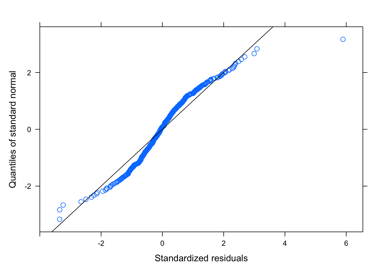
Diagnostics, model building
plot(shaf.lme)

qqnorm(shaf.lme, abline = c(0, 1))
Least squares means
# for cultivar
(lme.means.cv <- emmeans(shaf.lme, "gen"))
## NOTE: Results may be misleading due to involvement in interactions
##  gen      emmean  SE df lower.CL upper.CL
##  Bienvenu   2432 112 92     2211     2654
##  Bridger    2314 112 92     2092     2536
##  Cascade    2184 112 92     1962     2406
##  Dwarf      2308 112 92     2087     2530
##  Glacier    2463 112 92     2242     2685
##  Jet        2304 112 92     2082     2525
##
## Results are averaged over the levels of: loc, Year
## Degrees-of-freedom method: containment
## Confidence level used: 0.95
# for location
(lme.means.loc <- emmeans(shaf.lme, "loc"))
## NOTE: Results may be misleading due to involvement in interactions
##  loc emmean  SE df lower.CL upper.CL
##  GGA   1682 329 92     1030     2335
##  ID    4217 261 92     3698     4736
##  KS    1120 476 92      174     2066
##  MS    2204 476 92     1258     3150
##  MT    3339 474 92     2398     4280
##  NC    1328 329 92      676     1981
##  NY    3139 476 92     2193     4085
##  OR    3292 329 92     2640     3945
##  SC    1819 261 92     1300     2338
##  TGA   1028 261 92      509     1547
##  TN    2543 476 92     1597     3490
##  TX     827 329 92      174     1479
##  VA    2282 328 92     1631     2932
##  WA    3861 261 92     3342     4380
##
## Results are averaged over the levels of: gen, Year
## Degrees-of-freedom method: containment
## Confidence level used: 0.95
# for cultivar means within each location
lme.means.int <- emmeans(shaf.lme, ~ gen | loc + Year)

# this code would produce location means within each cultivar
# emmeans(model.lme, ~ loc | gen))
# also:
# emmeans(model.lme, ~ loc | gen)) provides the same estimates as 'emmeans(model.lme, ~ gen | loc))'
Pairwise Contrasts:
# all pairwise
pairs(lme.means.cv)
##  contrast           estimate   SE  df t.ratio p.value
##  Bienvenu - Bridger   118.57 87.6 470   1.353  0.7548
##  Bienvenu - Cascade   248.34 87.6 470   2.834  0.0539
##  Bienvenu - Dwarf     124.11 87.6 470   1.417  0.7170
##  Bienvenu - Glacier   -31.00 87.6 470  -0.354  0.9993
##  Bienvenu - Jet       128.70 87.6 470   1.469  0.6843
##  Bridger - Cascade    129.77 87.6 470   1.481  0.6765
##  Bridger - Dwarf        5.54 87.6 470   0.063  1.0000
##  Bridger - Glacier   -149.57 87.6 470  -1.707  0.5277
##  Bridger - Jet         10.13 87.6 470   0.116  1.0000
##  Cascade - Dwarf     -124.23 87.6 470  -1.418  0.7161
##  Cascade - Glacier   -279.34 87.6 470  -3.188  0.0190
##  Cascade - Jet       -119.64 87.6 470  -1.366  0.7477
##  Dwarf - Glacier     -155.10 87.6 470  -1.770  0.4861
##  Dwarf - Jet            4.59 87.6 470   0.052  1.0000
##  Glacier - Jet        159.70 87.6 470   1.823  0.4521
##
## Results are averaged over the levels of: loc, Year
## Degrees-of-freedom method: containment
## P value adjustment: tukey method for comparing a family of 6 estimates
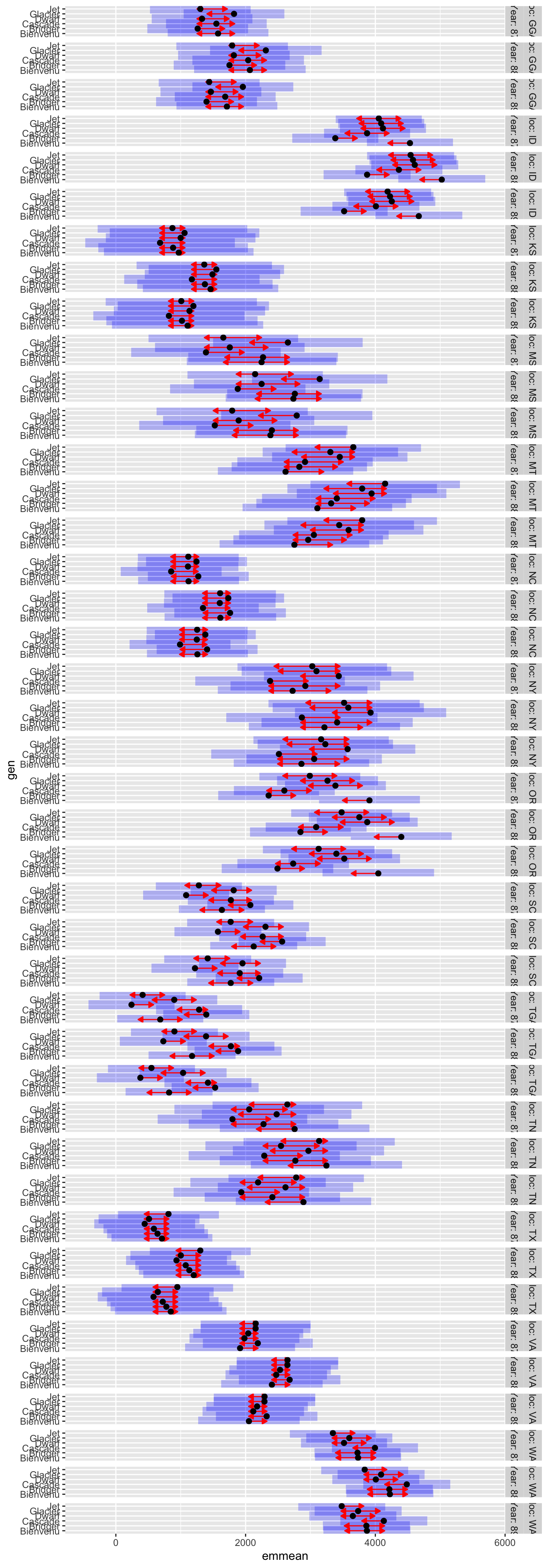
# plot results
plot(lme.means.cv, comparison = T)

plot(lme.means.loc, comparison = T, horizontal = F) # rotate plots to vertical position
## Warning: Comparison discrepancy in group "1", GGA - OR:
##     Target overlap = 0.0083, overlap on graph = -0.0111

# blue bars = lsmeans confidence 95% confidence intervals
# red arrows. pairwise differences (overlapping arrows = not significantly different)
For those who want the letters assigned to treatments based on all pairwise comparisons, it’s an unwieldy road:
library(multcomp) # this will need to be installed if you do not already have it
tukey <- glht(shaf.lme, linfct = mcp(loc = "Tukey"))
### extract information
cld_tukey <- cld(tukey)
print(cld_tukey)
##  GGA   ID   KS   MS   MT   NC   NY   OR   SC  TGA   TN   TX   VA   WA
##  "a"  "b"  "a" "ac" "ab"  "a" "ab" "bc"  "a"  "a" "ab"  "a"  "a" "bc"
Interaction plots can also be done:
(but, it gets unwieldy)
plot(lme.means.int, comparison = T, adjust = "tukey")
Other pre-set contrasts
# compare to a control, e.g. "Bridger"
levels(shafii.rapeseed$gen)
## [1] "Bienvenu" "Bridger" "Cascade" "Dwarf" "Glacier" "Jet"
# Bridger is listed in position 2 of the factor 'shafii.rapeseed$gen'
# so '2' is set as the reference level in the following contrast statement:

# "trt.vs.ctrlk" (treatment versus control treatment k) is a specific option to compare all treatment levels to a user-defined level
# by default, it will use the last level as the reference level

contrast(lme.means.cv, "trt.vs.ctrlk", ref = 2)
##  contrast           estimate   SE  df t.ratio p.value
##  Bienvenu - Bridger   118.57 87.6 470   1.353  0.5118
##  Cascade - Bridger   -129.77 87.6 470  -1.481  0.4315
##  Dwarf - Bridger       -5.54 87.6 470  -0.063  0.9998
##  Glacier - Bridger    149.57 87.6 470   1.707  0.3034
##  Jet - Bridger        -10.13 87.6 470  -0.116  0.9990
##
## Results are averaged over the levels of: loc, Year
## Degrees-of-freedom method: containment
## P value adjustment: dunnettx method for 5 tests
Search ?contrast.emmGrid to see full list of options for preset contrasts.
Custom contrasts
# example: contrast Western locations versus Southern locations

# first, find out what levels are present
unique(shafii.rapeseed$loc)
##  [1] GGA ID  KS  MS  MT  NC  NY  OR  SC  TGA TN  TX  VA  WA
## Levels: GGA ID KS MS MT NC NY OR SC TGA TN TX VA WA
# next create a contrast list
# this is a list of coefficients as long your list of treatment levels
# indicating what coefficients to give each treatment level

# in this example, levels "ID", "MT", "OR", and "WA" are contrasted versus
# "NC", "SC", "MS", "TN", "TX" and "VA"

cList <- list(West_V_South = c(0, 1/4, 0, -1/6, 1/4, -1/6, 0, 1/4, -1/6, 0, -1/6, -1/6, -1/6, 1/4))

# check that each contrast sums to zero:
lapply(cList, sum)
## $West_V_South
## [1] 5.551115e-17
lme.means.loc2 <- emmeans(shaf.lme, "loc", contr = cList)
## NOTE: Results may be misleading due to involvement in interactions
summary(lme.means.loc2)
## $emmeans
##  loc emmean  SE df lower.CL upper.CL
##  GGA   1682 329 92     1030     2335
##  ID    4217 261 92     3698     4736
##  KS    1120 476 92      174     2066
##  MS    2204 476 92     1258     3150
##  MT    3339 474 92     2398     4280
##  NC    1328 329 92      676     1981
##  NY    3139 476 92     2193     4085
##  OR    3292 329 92     2640     3945
##  SC    1819 261 92     1300     2338
##  TGA   1028 261 92      509     1547
##  TN    2543 476 92     1597     3490
##  TX     827 329 92      174     1479
##  VA    2282 328 92     1631     2932
##  WA    3861 261 92     3342     4380
##
## Results are averaged over the levels of: gen, Year
## Degrees-of-freedom method: containment
## Confidence level used: 0.95
##
## $contrasts
##  contrast     estimate  SE df t.ratio p.value
##  West_V_South     1843 233 92   7.910  <.0001
##
## Results are averaged over the levels of: gen, Year
## Degrees-of-freedom method: containment
# same contrast can also be done within each level of 'gen':
emmeans(shaf.lme, ~ loc | gen, contr = cList)
## $emmeans
## gen = Bienvenu:
##  loc emmean  SE df lower.CL upper.CL
##  GGA   1785 379 92  1032.31     2537
##  ID    4742 303 92  4140.13     5345
##  KS    1179 546 92    94.60     2263
##  MS    2455 546 92  1371.47     3539
##  MT    2825 544 92  1745.38     3904
##  NC    1330 379 92   577.36     2082
##  NY    2934 546 92  1849.69     4018
##  OR    4118 379 92  3365.98     4870
##  SC    1844 303 92  1241.42     2446
##  TGA    893 303 92   290.99     1496
##  TN    2965 546 92  1880.59     4049
##  TX     919 379 92   167.04     1671
##  VA    2124 378 92  1373.34     2875
##  WA    3943 303 92  3340.44     4545
##
## gen = Bridger:
##  loc emmean  SE df lower.CL upper.CL
##  GGA   1470 379 92   718.17     2223
##  ID    3591 303 92  2989.15     4194
##  KS    1091 546 92     7.35     2175
##  MS    2478 546 92  1393.89     3562
##  MT    3037 544 92  1957.63     4117
##  NC    1479 379 92   727.28     2232
##  NY    3130 546 92  2045.60     4214
##  OR    2564 379 92  1811.99     3316
##  SC    2282 303 92  1679.58     2884
##  TGA   1603 303 92  1000.66     2205
##  TN    2485 546 92  1401.33     3569
##  TX     851 379 92    99.08     1604
##  VA    2397 378 92  1646.76     3148
##  WA    3935 303 92  3332.27     4537
##
## gen = Cascade:
##  loc emmean  SE df lower.CL upper.CL
##  GGA   1758 379 92  1006.25     2511
##  ID    4081 303 92  3479.04     4684
##  KS     891 546 92  -193.40     1975
##  MS    1598 546 92   514.04     2682
##  MT    3125 544 92  2045.63     4205
##  NC    1062 379 92   309.61     1814
##  NY    2586 546 92  1502.21     3670
##  OR    2806 379 92  2053.82     3558
##  SC    1982 303 92  1379.70     2584
##  TGA   1492 303 92   889.83     2094
##  TN    2006 546 92   922.37     3090
##  TX     796 379 92    43.59     1548
##  VA    2191 378 92  1440.56     2942
##  WA    4203 303 92  3600.69     4805
##
## gen = Dwarf:
##  loc emmean  SE df lower.CL upper.CL
##  GGA   1538 379 92   785.71     2290
##  ID    4326 303 92  3723.81     4928
##  KS    1208 546 92   123.85     2292
##  MS    1966 546 92   881.69     3050
##  MT    3661 544 92  2581.14     4740
##  NC    1321 379 92   568.53     2073
##  NY    3645 546 92  2561.26     4729
##  OR    3594 379 92  2841.40     4346
##  SC    1292 303 92   690.10     1895
##  TGA    451 303 92  -151.81     1053
##  TN    2688 546 92  1603.57     3771
##  TX     654 379 92   -98.64     1406
##  VA    2250 378 92  1499.12     3000
##  WA    3726 303 92  3123.52     4328
##
## gen = Glacier:
##  loc emmean  SE df lower.CL upper.CL
##  GGA   2031 379 92  1278.35     2783
##  ID    4299 303 92  3696.61     4901
##  KS    1268 546 92   183.85     2352
##  MS    2861 546 92  1776.82     3945
##  MT    3516 544 92  2436.14     4595
##  NC    1452 379 92   699.82     2204
##  NY    3301 546 92  2217.49     4385
##  OR    3472 379 92  2719.36     4224
##  SC    2025 303 92  1422.97     2628
##  TGA   1109 303 92   506.90     1712
##  TN    2265 546 92  1180.58     3348
##  TX     720 379 92   -31.85     1473
##  VA    2363 378 92  1612.64     3114
##  WA    3807 303 92  3205.02     4410
##
## gen = Jet:
##  loc emmean  SE df lower.CL upper.CL
##  GGA   1511 379 92   758.95     2263
##  ID    4262 303 92  3659.68     4864
##  KS    1082 546 92    -2.40     2166
##  MS    1866 546 92   781.68     2950
##  MT    3869 544 92  2789.89     4949
##  NC    1326 379 92   573.58     2078
##  NY    3237 546 92  2152.80     4321
##  OR    3199 379 92  2446.70     3951
##  SC    1488 303 92   886.13     2091
##  TGA    622 303 92    19.27     1224
##  TN    2853 546 92  1768.63     3937
##  TX    1020 379 92   267.99     1772
##  VA    2364 378 92  1613.85     3115
##  WA    3554 303 92  2952.19     4157
##
## Results are averaged over the levels of: Year
## Degrees-of-freedom method: containment
## Confidence level used: 0.95
##
## $contrasts
## gen = Bienvenu:
##  contrast     estimate  SE df t.ratio p.value
##  West_V_South     1968 267 92   7.359  <.0001
##
## gen = Bridger:
##  contrast     estimate  SE df t.ratio p.value
##  West_V_South     1286 267 92   4.811  <.0001
##
## gen = Cascade:
##  contrast     estimate  SE df t.ratio p.value
##  West_V_South     1948 267 92   7.286  <.0001
##
## gen = Dwarf:
##  contrast     estimate  SE df t.ratio p.value
##  West_V_South     2132 267 92   7.972  <.0001
##
## gen = Glacier:
##  contrast     estimate  SE df t.ratio p.value
##  West_V_South     1826 267 92   6.828  <.0001
##
## gen = Jet:
##  contrast     estimate  SE df t.ratio p.value
##  West_V_South     1902 267 92   7.112  <.0001
##
## Results are averaged over the levels of: Year
## Degrees-of-freedom method: containment
To perform custom contrasts on a another variable, a cList and emmeans call for that variable is required.
ANCOVA
(analysis of covariance) From a R programming perspective, this is no different than running a standard linear model. A data set from agridat, “theobald.covariate” comparing corn silage yields across multiple years, locations and cultivars. The data set includes a covariate, “chu” (corn heat units, a bit like growing degree days).
Load data and examine:
data(theobald.covariate)
str(theobald.covariate)
## 'data.frame':	256 obs. of  5 variables:
##  $ year : int  1990 1990 1990 1990 1990 1991 1991 1991 1991 1991 ...
##  $ env  : Factor w/ 7 levels "E1","E2","E3",..: 1 2 3 4 7 1 2 3 4 5 ...
##  $ gen  : Factor w/ 10 levels "G01","G02","G03",..: 1 1 1 1 1 1 1 1 1 1 ...
##  $ yield: num  6.27 5.57 8.45 7.35 6.5 6.71 5.59 8.36 7.25 8.09 ...
##  $ chu  : num  2.57 2.53 2.72 2.72 2.48 2.44 2.55 2.75 2.75 2.61 ...
count_na(theobald.covariate)
##  year   env   gen yield   chu
##     0     0     0     0     0
Exploratory plots:
# distributions of continuous variables
hist(theobald.covariate$yield, col = "gold")

hist(theobald.covariate$chu, col = "gray70")

# relationship between reponse variable and covariate:
with(theobald.covariate, plot(chu, yield))

length(unique(theobald.covariate$chu))
## [1] 21
# the usual boxplots:
boxplot(yield ~ env, data = theobald.covariate, col = "orangered")

boxplot(yield ~ year, data = theobald.covariate, col = "chartreuse")

boxplot(yield ~ gen, data = theobald.covariate, col = "darkcyan")

Check the extent of replication:
theobald.covariate$Year <- as.factor(theobald.covariate$year)
replications(yield ~ Year + env + gen, data = theobald.covariate)
## $Year
## Year
## 1990 1991 1992 1993 1994
##   40   63   60   45   48
##
## $env
## env
## E1 E2 E3 E4 E5 E6 E7
## 35 35 44 36 36 36 34
##
## $gen
## gen
## G01 G02 G03 G04 G05 G06 G07 G08 G09 G10
##  29  29  29  29  22  29  23  18  24  24
# with(theobald.covariate, table(gen, env, Year)) # lots of useful output
The treatments are not fully crossed, so a fully specified model of the form yield ~ Year*env*gen*chu cannot be tested. The treatments and interactions were tested in reduced models and compared (not shown). The final “best” model is shown below.
# the covariate, chu, is added in like any other effect.
theobald.lm2 <- lm(yield ~  Year + env*chu, data = theobald.covariate)
Anova(theobald.lm2, type = "III")
## Anova Table (Type III tests)
##
## Response: yield
##              Sum Sq  Df F value    Pr(>F)
## (Intercept)   4.309   1  6.8321  0.009524 **
## Year         76.589   4 30.3607 < 2.2e-16 ***
## env          13.473   6  3.5607  0.002138 **
## chu          11.831   1 18.7596 2.187e-05 ***
## env:chu      13.376   6  3.5350  0.002268 **
## Residuals   150.096 238
## ---
## Signif. codes:  0 '***' 0.001 '**' 0.01 '*' 0.05 '.' 0.1 ' ' 1
# how to extract the covariate slope(s):
emtrends(theobald.lm2, ~ env, "chu")
##  env chu.trend   SE  df lower.CL upper.CL
##  E1      7.015 1.62 238     3.82    10.21
##  E2      0.979 4.44 238    -7.76     9.72
##  E3      4.099 3.15 238    -2.11    10.31
##  E4     -2.884 3.54 238    -9.87     4.10
##  E5      8.222 2.70 238     2.90    13.54
##  E6      3.425 2.72 238    -1.93     8.78
##  E7     -0.359 2.55 238    -5.38     4.66
##
## Results are averaged over the levels of: Year
## Confidence level used: 0.95
# emmeans extracted as usual:
emmeans(theobald.lm2, ~ env)
## NOTE: Results may be misleading due to involvement in interactions
##  env emmean    SE  df lower.CL upper.CL
##  E1    6.67 0.175 238     6.32     7.01
##  E2    5.13 0.256 238     4.63     5.64
##  E3    6.66 0.482 238     5.71     7.61
##  E4    7.22 0.508 238     6.22     8.22
##  E5    6.61 0.138 238     6.34     6.88
##  E6    6.43 0.236 238     5.97     6.90
##  E7    6.32 0.397 238     5.54     7.10
##
## Results are averaged over the levels of: Year
## Confidence level used: 0.95
emmeans(theobald.lm2, ~ Year)
##  Year emmean    SE  df lower.CL upper.CL
##  1990   6.97 0.189 238     6.60     7.34
##  1991   6.75 0.170 238     6.41     7.08
##  1992   7.07 0.187 238     6.70     7.44
##  1993   5.39 0.208 238     4.98     5.80
##  1994   6.00 0.218 238     5.57     6.43
##
## Results are averaged over the levels of: env
## Confidence level used: 0.95
Split-plot
Load “Oats” from nlme. Nitrogen level (“nitro”) is the main plot, cultivar (“Variety”) is the sub-plot and “Block” describes the blocking layout.
data(Oats)
str(Oats)
## Classes 'nfnGroupedData', 'nfGroupedData', 'groupedData' and 'data.frame':	72 obs. of  4 variables:
##  $ Block  : Ord.factor w/ 6 levels "VI"<"V"<"III"<..: 6 6 6 6 6 6 6 6 6 6 ...
##  $ Variety: Factor w/ 3 levels "Golden Rain",..: 3 3 3 3 1 1 1 1 2 2 ...
##  $ nitro  : num  0 0.2 0.4 0.6 0 0.2 0.4 0.6 0 0.2 ...
##  $ yield  : num  111 130 157 174 117 114 161 141 105 140 ...
##  - attr(*, "formula")=Class 'formula'  language yield ~ nitro | Block
##   .. ..- attr(*, ".Environment")=<environment: R_GlobalEnv>
##  - attr(*, "labels")=List of 2
##   ..$ y: chr "Yield"
##   ..$ x: chr "Nitrogen concentration"
##  - attr(*, "units")=List of 2
##   ..$ y: chr "(bushels/acre)"
##   ..$ x: chr "(cwt/acre)"
##  - attr(*, "inner")=Class 'formula'  language ~Variety
##   .. ..- attr(*, ".Environment")=<environment: R_GlobalEnv>
count_na(Oats)
##   Block Variety   nitro   yield
##       0       0       0       0
Oats$N <- as.factor(Oats$nitro)
replications(yield ~ Variety*N*Block, data = Oats)
##         Variety               N           Block       Variety:N   Variety:Block
##              24              18              12               6               4
##         N:Block Variety:N:Block
##               3               1
table(Oats$Variety, Oats$N)
##
##               0 0.2 0.4 0.6
##   Golden Rain 6   6   6   6
##   Marvellous  6   6   6   6
##   Victory     6   6   6   6
hist(Oats$yield, col = "gold")

boxplot(yield ~ N, data = Oats, col = "dodgerblue1")

boxplot(yield ~ Variety, data = Oats, col = "red3")

Balanced Trial Analysis
The format for specifying split-plot error terms is Error(blocking factor/main plot).
#contrasts("contr.sum")
spl.oats <- aov(yield ~ Variety*N + Error(Block:N), data = Oats)
summary(spl.oats)
##
## Error: Block:N
##           Df Sum Sq Mean Sq F value  Pr(>F)
## N          3  20020    6673   7.556 0.00143 **
## Residuals 20  17663     883
## ---
## Signif. codes:  0 '***' 0.001 '**' 0.01 '*' 0.05 '.' 0.1 ' ' 1
##
## Error: Within
##           Df Sum Sq Mean Sq F value Pr(>F)
## Variety    2   1786   893.2   2.930 0.0649 .
## Variety:N  6    322    53.6   0.176 0.9818
## Residuals 40  12194   304.8
## ---
## Signif. codes:  0 '***' 0.001 '**' 0.01 '*' 0.05 '.' 0.1 ' ' 1
emmeans(spl.oats, "N")
## Note: re-fitting model with sum-to-zero contrasts
## NOTE: Results may be misleading due to involvement in interactions
##  N   emmean SE df lower.CL upper.CL
##  0     79.4  7 20     64.8       94
##  0.2   98.9  7 20     84.3      114
##  0.4  114.2  7 20     99.6      129
##  0.6  123.4  7 20    108.8      138
##
## Results are averaged over the levels of: Variety
## Warning: EMMs are biased unless design is perfectly balanced
## Confidence level used: 0.95
emmeans(spl.oats, ~ Variety)
## Note: re-fitting model with sum-to-zero contrasts
## NOTE: Results may be misleading due to involvement in interactions
##  Variety     emmean   SE   df lower.CL upper.CL
##  Golden Rain  104.5 4.55 46.1     95.3      114
##  Marvellous   109.8 4.55 46.1    100.6      119
##  Victory       97.6 4.55 46.1     88.5      107
##
## Results are averaged over the levels of: N
## Warning: EMMs are biased unless design is perfectly balanced
## Confidence level used: 0.95
Unbalanced Trial Analysis
spl.oats2 <- lmer(yield ~ N*Variety + (1|Block:N), data = Oats)
Anova(spl.oats2, type = "3")
## Analysis of Deviance Table (Type III Wald chisquare tests)
##
## Response: yield
##               Chisq Df Pr(>Chisq)
## (Intercept) 77.1670  1  < 2.2e-16 ***
## N           13.9028  3   0.003041 **
## Variety      2.2747  2   0.320663
## N:Variety    1.0554  6   0.983423
## ---
## Signif. codes:  0 '***' 0.001 '**' 0.01 '*' 0.05 '.' 0.1 ' ' 1
emmeans(spl.oats2, "N")
## NOTE: Results may be misleading due to involvement in interactions
##  N   emmean SE df lower.CL upper.CL
##  0     79.4  7 20     64.8       94
##  0.2   98.9  7 20     84.3      114
##  0.4  114.2  7 20     99.6      129
##  0.6  123.4  7 20    108.8      138
##
## Results are averaged over the levels of: Variety
## Degrees-of-freedom method: kenward-roger
## Confidence level used: 0.95
emmeans(spl.oats2, ~ Variety)
## NOTE: Results may be misleading due to involvement in interactions
##  Variety     emmean   SE   df lower.CL upper.CL
##  Golden Rain  104.5 4.55 46.1     95.3      114
##  Marvellous   109.8 4.55 46.1    100.6      119
##  Victory       97.6 4.55 46.1     88.5      107
##
## Results are averaged over the levels of: N
## Degrees-of-freedom method: kenward-roger
## Confidence level used: 0.95
Other Designs
There are many other experimental designs commonly used in agricultural trials (split-split plot, split-block, alpha lattice, etc). We have written an online resource for routine incorporation of spatial covariates into field trial analysis that includes information on how to analyze different designs. You could also consider using the agricolae package.
Extra Functions
for extracting model parameters, diagnostics and other model information
These work differently with different R object types. That is, different output will result depending on if a “lm”, “lme” or “merMod” (lmer) object is used in the function call.
# extract model summary
summary()

#extract coefficients:
coef()

#extract residuals
resid()
rstudent()
residuals()

# extract predicted values
fits()

# make diagnostic plots
plot()

# extract influence measures:
influence.measures()

#other fir diagnostics:
cooks.distance()
dffits()
dfbeta()
hat()
To see the all functions available for a particular type of linear model object, use:
methods(class = "lm") # for lm objects
##  [1] add1                addterm             alias
##  [4] anova               Anova               attrassign
##  [7] avPlot              Boot                bootCase
## [10] boxcox              boxCox              brief
## [13] case.names          ceresPlot           coerce
## [16] concordance         confidenceEllipse   confint
## [19] Confint             cooks.distance      crPlot
## [22] deltaMethod         deviance            dfbeta
## [25] dfbetaPlots         dfbetas             dfbetasPlots
## [28] drop1               dropterm            dummy.coef
## [31] durbinWatsonTest    effects             emm_basis
## [34] extractAIC          family              formula
## [37] hatvalues           hccm                infIndexPlot
## [40] influence           influencePlot       initialize
## [43] inverseResponsePlot kappa               labels
## [46] leveneTest          leveragePlot        linearHypothesis
## [49] logLik              logtrans            mcPlot
## [52] mmp                 model.frame         model.matrix
## [55] ncvTest             nextBoot            nobs
## [58] outlierTest         plot                powerTransform
## [61] predict             Predict             print
## [64] proj                qqnorm              qqPlot
## [67] qr                  recover_data        residualPlot
## [70] residualPlots       residuals           rstandard
## [73] rstudent            S                   show
## [76] sigmaHat            simulate            slotsFromS3
## [79] spreadLevelPlot     summary             symbox
## [82] variable.names      vcov
## see '?methods' for accessing help and source code
methods(class = "lme") # for lme4 objects
##  [1] ACF              anova            Anova            augPred
##  [5] coef             comparePred      confint          Confint
##  [9] deltaMethod      deviance         emm_basis        extractAIC
## [13] fitted           fixef            formula          getData
## [17] getGroups        getGroupsFormula getResponse      getVarCov
## [21] influence        intervals        linearHypothesis logLik
## [25] matchCoefs       nobs             pairs            plot
## [29] predict          print            qqnorm           ranef
## [33] recover_data     residuals        S                sigma
## [37] simulate         summary          update           VarCorr
## [41] Variogram        vcov
## see '?methods' for accessing help and source code
methods(class = "merMod") # for nlme objects
##  [1] anova            Anova            as.function      coef
##  [5] confint          cooks.distance   deltaMethod      deviance
##  [9] df.residual      drop1            emm_basis        extractAIC
## [13] family           fitted           fixef            formula
## [17] getData          getL             getME            hatvalues
## [21] influence        isGLMM           isLMM            isNLMM
## [25] isREML           linearHypothesis logLik           matchCoefs
## [29] model.frame      model.matrix     na.action        ngrps
## [33] nobs             plot             predict          print
## [37] profile          ranef            recover_data     refit
## [41] refitML          rePCA            residuals        rstudent
## [45] show             sigma            simulate         summary
## [49] terms            update           VarCorr          vcov
## [53] vif              weights
## see '?methods' for accessing help and source code
The package emmeans also supports a large number of models.
Julia Piaskowski
Statistician
My research interests include plant genetics, spatial statistics and how to implement open science and reproducible research practices routinely.